Variational Autoencoders
Introduction
In this article, I will delve into the theoretical foundations of Variational Autoencoders (VAE). You can find the code used for both Convolutional Neural Network (CNN) and normal feedforward autoencoder trained on the MNIST dataset on my GitHub repository.
VAEs are generative models grounded in Bayesian inference theory and variational inference. The underlying concept involves generating data points from a given latent variable that encodes the characteristics of the desired data. To illustrate, consider the task of dwaring an animal. Initially, we conceptualize the animal with specific criteria, such as having four legs and the ability to swim. With these criteria, we can draw the animal by sampling from the animal kingdom.
Let use define some notation:
- \(x\) represents a data point.
- \(z\) is a latent variable.
- \(p(x)\) denotes the probability distribution of the data.
- \(p(z)\) signifies the probability of the latent variable indicating the type of generated data.
- \(p(x|z)\) represents the distribution of the generated data based on a latent variable. Analogously, it is akin to transforming imagination into reality.
- \(D_{KL}\big(p(X) \parallel q(X)\big) = \sum_{x_i \in X} p(x_i) \log \frac{p(x_i)}{q(x_i)} = - \sum_{x_i \in X} p(x_i) \log \frac{q(x_i)}{p(x_i)}\) is the Kullback-Leibler (KL) divergence between two discrete distributions.
KL divergence possesses notable properties: firstly, \(D_{KL}\big(p(x) \parallel q(x)\big)\) is not equal to \(D_{KL}\big(q(x) \parallel p(x)\big)\), indicating its asymmetric nature. Secondly, \(D_{KL} > 0\).
Variationa Autoencoders
Variational Autoencoders function as generative models, enabling the sampling of new data points from such a model. In general, generative models learn a functional form of \(p(x)\) that allows for sampling. However, \(p(x)\)is often unknown, and only a dataset \(\hat{X} = (x_i)^N_{i=1}\) comprising some samples from \(p(x)\) is provided.
VAEs overcome this challenge by leveraging the concept that high-dimensional data is generated based on a low-dimensional latent variable \(z\); thus, the joint distribution can be factorized as \(p(x,z)=p(x∣z)p(z)\). Ultimately, through marginalization, we can define \(p(x)\) as:
\[ p(x) = \int p(x|z) p(z) \partial z. \]
In our earlier analogy, \(z\) represents the imagined concept, while \(x\) is the realization of all the selected concepts. As mentioned before, during the training phase of VAEs, access is neither given to \(p(x)\) nor to the latent variable \(z\) used to generate the dataset. However, throughout the training process, a reasonable posterior distribution \(p(z∣x)\) is learned. This approach makes sense, as the goal is to make the latent variable likely under the observed data, thereby generating plausible data.
According to Bayesian theory:
\[ p(z|x) = \frac{p(x|z)\cdot p(z)}{p(x)} = \frac{p(x, z)}{p(x)}. \]
As mentioned earlier, \(p(x)\) can be expressed through marginalization over \(z\); however, such computation is typically intractable as it involves integrating over all latent dimensions:
\[ p(x) \int ... \int \int p(x|z)\cdot p(z) \partial z_i. \]
To overcome this computational challenge, variational inference suggests approximating \(p(z∣x)\) with a simpler distribution \(q(z∣x)\). By assigning a tractable form to \(q(z∣x)\), such as a Gaussian distribution, and adjusting its parameters to closely match \(p(z∣x)\), we can overcome the intractability issue.
Formally, we can rewrite our goal as: \[ \begin{align*} \min D_{KL}\big(q(z|x) || p(z|x)\big) & = - \sum_{x \in \hat{X}} q(z|x) \log \frac{p(z|x)}{q(z|x)} \\ & = - \sum_{x \in \hat{X}} q(z|x) \log \Big(\frac{p(x, z)}{q(z|x)} \cdot \frac{1}{p(x)} \Big) \\ & = - \sum_{x \in \hat{X}} q(z|x) \log \Big(\frac{p(x, z)}{q(z|x)} - \log p(x) \Big) \\ & = - \sum_{x \in \hat{X}} q(z|x) \log \frac{p(x, z)}{q(z|x)} + \sum_{x \in \hat{X}} q(z|x) \log p(x) \\ & = \log p(x) - \sum_{x \in \hat{X}} q(z|x) \log \frac{p(x, z)}{q(z|x)} ~~~~ \small{\text{:as $\sum_{x \in \hat{X}} q(z|x) = 1$ and $p(x)$ do not depend on $z$}} \end{align*} \]
By rearranging the above equation we can state that: \[ \log p(x) = D_{KL}\big(q(z|x) || p(z|x)\big) + \sum_{x \in \hat{X}} q(z|x) \log \frac{p(x, z)}{q(z|x)}. \]
However, \(p(x)\) is constant for a given dataset \(\hat{X}\), thus minimizing \(D_{KL}\big(q(z|x) || p(z|x)\big)\) is equivalent to maximise \(\sum_{x \in \hat{X}} q(z|x) \log \frac{p(x, z)}{q(z|x)}\) up to a constant factor. Such formulation of the KL-divergenve is also known as the Evidence Lower Bound (ELBO) and it is tractable:
\[ \begin{align*} \sum_{x \in \hat{X}} q(z|x) \log \frac{p(x, z)}{q(z|x)} & = \sum_{x \in \hat{X}} q(z|x) \log \big( \frac{p(x|z) p(z)}{q(z|x)}\big) \\ & = \sum_{x \in \hat{X}} q(z|x) \Big(\log p(x|z) + \log \frac{p(z)}{q(z|x)} \Big) \\ & = \sum_{x \in \hat{X}} q(z|x) \log p(x|z) + \sum_{x \in \hat{X}} q(z|x) \log \frac{p(z)}{q(z|x)} \\ & = \mathbb{E}_{z \sim q(z|x)} \big[ \log p(x|z) \big] - \sum_{x \in \hat{X}} q(z|x) \log \frac{q(z|x)}{p(z)} \\ & = \mathbb{E}_{z \sim q(z|x)} \big[ \log p(x|z) \big] - \mathbb{E}_{z \sim q(z|x)} \big[ \log q(z|x) - \log p(z) \big] \\ & = \mathbb{E}_{z \sim q(z|x)} \big[ \log p(x|z) \big] - D_{KL}\big( q(z|x) \parallel p(z) \big). \end{align*} \]
The initial component of the ELBO, denoted as \(\mathbb{E}_{z \sim q(z|x)} \big[ \log p(x|z) \big]\) , is commonly known as the (negative) reconstruction error. This is because it involves encoding \(x\) into \(z\) and then decoding it back. The second segment, \(D_{KL}\big( q(z|x)\parallel p(z) \big)\) can be viewed as a regularization term that imposes a specific distribution on \(q\).
Results
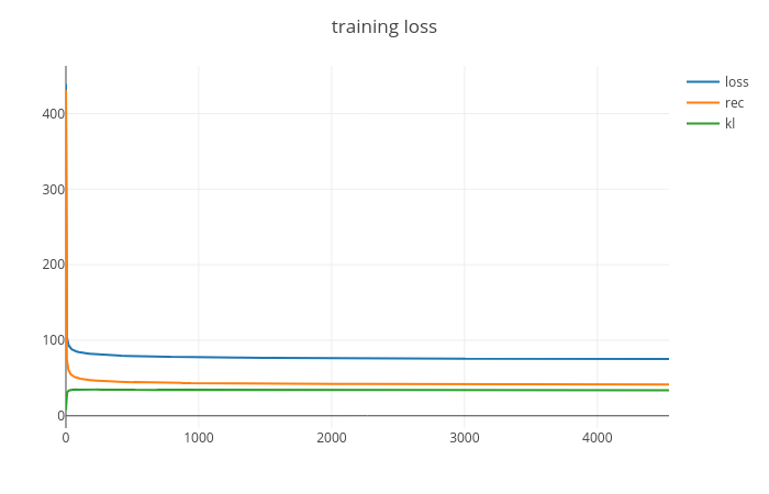
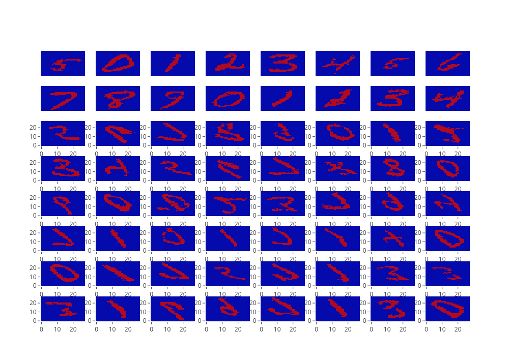
Based on the code, we have trained a CNN-based Variational Autoencoder on the MNIST dataset. Figure 1 report the training loss, while Figure 2 shows us some generated example. As it is possible to see, there are still some artifact. Maybe a better activation function would provide better results.

