Normalizing Flows
Normalizing Flows (NF) represent a potent technique that facilitates the learning and sampling from intricate probability distributions [1] [2]. These models, categorized as generative models, enable the precise estimation of likelihood for continuous input data, denoted as \(p(x)\). In contrast to methods such as variational inference that rely on approximations, normalizing flows function by transforming samples from a simple distribution, denoted as \(z \sim p(z)\), into samples from a more complex distribution using the following transformation:
\[ x = f_{\theta}(z), ~~ z \sim p(z; \psi). \]
Here, \(f_{\theta}(\cdot)\) is a mapping function from \(z\) to \(x\), parametrized by \(\theta\), and \(p(z; \psi)\) is the base distribution (sometimes referred to as the prior distribution), parametrized by \(\psi\), from which samples can be drawn. The essential properties defining a normalizing flow include:
The defining propertires of a normalizing flow are:
- \(f_{\theta}(\cdot)\) must be invertible,
- Both \(f_{\theta}(\cdot)\) and \(f_{\theta}^{-1}(\cdot)\) must be differentiable.
Adhering to these constraints ensures the well-defined density of \(x\), as established by the change-of-variable theorem [3]:
\[ \begin{align*} \int p(x) \partial x &= \int p(z) \partial z = 1 \\ \implies p(x) & = p(z) \cdot |\frac{\partial z}{\partial x}| \\ & = p\big(f_{\theta}^{-1}(x)\big) \cdot |\frac{\partial f_{\theta}^{-1}(x)}{\partial x}| \\ \end{align*} \]
In its definition, \(\partial x\) represents the width of an infinitesimally small rectangle with height \(p(x)\). Consequently, \(\frac{\partial f_{\theta}^{-1}(x)}{\partial x}\) denotes the ratio between the areas of rectangles defined in two distinct coordinate systems: one in terms of \(x\) and the other in terms of \(z\).
For illustrative purposes, consider Figure 1, which depicts how the affine transformation \(f_{\theta}^{-1}(x) = (5 \cdot x) - 2\) maps the Normal distribution \(p(x; \mu=0, \sigma=1)\) to another Gaussian distribution \(p(z; \mu=-2, \sigma=5)\). With \(\frac{\partial z}{\partial x} = 5\), the area \(\partial x\) undergoes a stretching factor of 5 when transformed into the variable \(z\). Consequently, \(p(z)\) must be lowered by a factor of 5 to maintain its validity as a probability density function, satisfying the condition \(\int p(z) \partial z = 1\):
\[ p(z) = \frac{p(x)}{\frac{\partial f_{\theta}^{-1}(x)}{\partial x}} = \frac{p(x)}{f_{\theta}^{-1'}(x)}. \]
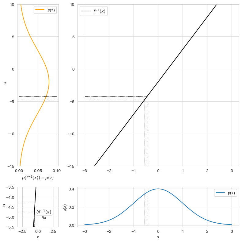
Take note of the disparity between the maximum values of \(p(z)\) and \(p(x)\) for a visual representation, as depicted in the lower-left image illustrating the stretching of \(\partial x\) caused by the transformation \(f_{\theta}^{-1}(\cdot)\).
In the preceding paragraph, we introduced the concept of area-preserving transformations. Extending this notion to the multidimensional space involves considering \(\frac{\partial z}{\partial x}\) not as a simple derivative but as the Jacobian matrix:
\[ J_{z}(x) = \begin{bmatrix} \frac{\partial z_1}{\partial x_1} & \dots & \frac{\partial z_1}{\partial x_D}\\ \vdots & \ddots & \vdots \\ \frac{\partial z_D}{\partial x_1} & \dots & \frac{\partial z_D}{\partial x_D} \end{bmatrix}. \]
In the multidimensional setting, the difference in areas translates to a difference in volumes quantified by the determinant of the Jacobian matrix, denoted as \(det(J_{z}(x)) \approx \frac{Vol(z)}{Vol(x)}\). Consolidating these concepts, we can formalize a multidimensional normalization flow as follows:
\[ \begin{align*} p(x) & = p(z) \cdot |det(\frac{\partial z}{\partial x})| \\ & = p(f_{\theta}^{-1}(x)) \cdot |det(\frac{\partial f_{\theta}^{-1}(x)}{\partial x})| \\ & = p(f_{\theta}^{-1}(x)) \cdot |det(J_{f_{\theta}^{-1}}(x))|. \end{align*} \]
Generative Process as Finate Composition of Transformations
In the general case, the transformations \(f_{\theta}(\cdot)\) and \(f_{\theta}^{-1}(\cdot)\) are defined as finite compositions of simpler transformations \(f_{\theta_i}\):
\[ \begin{align*} x & = z_{K} = f_{\theta}(z_0) = f_{\theta_K} \dots f_{\theta_2} \circ f_{\theta_1}(z_0) & \\ p(x) & = p_K(z_{k}) = p_{K-1}(f_{\theta_K}^{-1}(z_{k})) \cdot \Big| det\Big(J_{f_{\theta_K}^{-1}}(z_{k})\Big)\Big| & \\ & = p_{K-1}(z_{K-1}) \cdot \Big| det\Big(J_{f_{\theta_K}^{-1}}(z_k)\Big)\Big| & \text{Due to the definition of } f_{\theta_K}(z_{K-1}) = z_K\\ & = p_{K-1}(z_{K-1}) \cdot \Big| det\Big( J_{f_{\theta_K}(z_{K-1})} \Big)^{-1}\Big| & \text{As: } J_{f_{\theta_K}^{-1}}(x) = \frac{f_{\theta_K}^{-1}(z_k)}{\partial z_K} \\ & & = \Big(\frac{\partial z_K}{\partial f_{\theta_k}^{-1}(z_k)} \Big)^{-1} \\ & & = \Big(\frac{\partial f_{\theta_{k}}(z_{K-1})}{\partial z_{K-1}}\Big)^{-1} \\ & & = \Big( J_{f_{\theta_K}(z_{K-1})} \Big)^{-1} \\ & = p_{K-1}(z_{K-1}) \cdot \Big| det\Big( J_{f_{\theta_K}}(z_{K-1}) \Big)\Big|^{-1}. \\ \end{align*} \]
By this process, \(p(z_i)\) is fully described by \(z_{i-1}\) and \(f_{\theta_i}\), allowing the extension of the previous reasoning to all i-steps of the overall generative process:
\[ \begin{equation} p(x) = p(z_0) \cdot \prod_{i=1}^k \Big| det \big( J_{f_{\theta_i}}(z_{i-1}) \big) \Big|^{-1}. \end{equation} \tag{1}\]
It is noteworthy that in the context of generative models, \(f_{\theta}\) is also referred to as a pushforward mapping from a simple density \(p(z)\) to a more complex \(p(x)\). On the other hand, the inverse transformation \(f_{\theta}^{-1}\) is known as the normalization function, as it systematically “normalizes” a complex distribution into a simpler one, one step at a time.
Training Procedures
As previously mentioned, NFs serve as efficient models for both sampling from and learning complex distributions. The primary applications of NFs lie in density estimation and data generation.
Density estimation proves valuable for computing statistical quantities over unseen data, as demonstrated in works such as [4] and [5], where NF models effectively estimate densities for tabular and image datasets. Additionally, NFs find application in anomaly detection [6], although requiring careful tuning for out-of-distribution detection [7].
On the flip side, data generation stands out as the central application for NFs. As mentioned earlier, NFs, under mild assumptions, can sample new data points from a complex distribution \(p(x)\). Exemplifying this, [8] showcases NFs applied to image generation, while [9] and [10] demonstrate successful learning of audio signals through NFs.
A key advantage of NFs over other probabilistic generative models lies in their ease of training, achieved by minimizing a divergence metric between \(p(x; \theta)\) and the target distribution \(p(x)\). In most cases, NFs are trained by minimizing the Kullback-Leibler (KL) divergence between these two distributions:
\[ \begin{align*} \mathcal{L}(\theta) & = D_{KL}[p(x) || p(x; \theta)] \\ & = - \sum_{x \sim p(x)} p(x) \cdot \log \frac{p(x; \theta)}{p(x)} \\ & = - \sum_{x \sim p(x)} p(x) \cdot \log p(x; \theta) + \sum_{x \sim p(x)} p(x) \cdot \log p(x) \\ & = - \mathbb{E}_{x \sim p(x)} \Big[ \log p(x; \theta) \Big] + \mathbb{E}_{x \sim p(x)} \Big[ \log p(x) \Big] \\ & = - \mathbb{E}_{x \sim p(x)}\Big[\log p(x; \theta)\Big] + const. ~~~ \text{As it does not depend on $\theta$} \\ & = - \mathbb{E}_{x \sim p(x)}\Big[\log p\big(f_{\theta}^{-1}(x)\big) + \sum_{i=1}^{K} \log \Big| det\big( J_{f_{\theta_i}^{-1}}(z_{i}) \big)\Big| \Big] + const. \end{align*} \]
Here, \(p(f_{\theta}^{-1}(x)) = p(z_0)\), and \(z_K\) is equal to \(x\). For a fixed training set \(X_N = \\{ x_n \\}_{n=1}^N\), the loss function is derived as the negative log-likelihood typically optimized using stochastic gradient descent:
\[ \begin{equation} \mathcal{L}(\theta) = - \frac{1}{N} \sum_{n=1}^N \log p\big(f_{\theta}^{-1}(x)\big) + \sum_{i=1}^{K} \log \Big| det\big( J_{f_{\theta_i}^{-1}}(z_{i}) \big)\Big|. \end{equation} \tag{2}\]
It is important to note that the loss function (Equation 2) is computed by starting from a datapoint \(x\) and reversing it to a plausible latent variable \(z_0\). Consequently, the structural formulation of \(p(z_0)\) plays a critical role in defining the training signals: if \(p(z_0)\) is too lax, the training process lacks substantial information; if it is too stringent, the training process may become overly challenging. Furthermore, the training process is the inverse of the generative process defined in Equation 1, emphasizing the importance of the sum of determinants. Achieving computationally efficient training requires the efficient computation of determinants of \(J_{f_{\theta_i}^{-1}}\). While auto-diff libraries can compute gradients with respect to \(\theta_i\) of the Jacobian matrix and its determinant, such computations are computationally expensive (\(O(n)^3\)). Therefore, significant research efforts have focused on designing transformations with efficient Jacobian determinant formulations.
Training Example
As previously mentioned, the training process of a NF involves mapping a given input data \(x\) to a specific base distribution \(p(z_0)\). Typically, the base distribution is a well-known distribution such as a multivariate Gaussian, Uniform, or any other exponential distribution. Similarly, the mapping function is usually implemented as a neural network.
Starting from first principles, any NF model can be specified as comprising a base distribution and a series of flows that map \(x\) to \(z_0\). Here is a Python implementation:
class NormalizingFlow(nn.Module):
    def __init__(
        self,
        prior: Distribution,
        flows: nn.ModuleList,
    ):
        super().__init__()
        self.prior = prior
        self.flows = flows

    def forward(self, x: Tensor):
        bs = x.size(0)
        zs = [x]
        sum_log_det = torch.zeros(bs).to(x.device)
        for flow in self.flows:
            z = flow(x)
            log_det = flow.log_abs_det_jacobian(x, z)
            zs.append(z)
            sum_log_det += log_det
            x = z

        prior_logprob = self.prior.log_prob(z).view(bs, -1).sum(-1)
        log_prob = prior_logprob + sum_log_det

        intermediat_results = dict(
            prior_logprob=prior_logprob,
            sum_log_det=sum_log_det,
            zs=zs,
        )
        return log_prob, intermediat_results
where the prior can be any base distribution inplemented in torch.distributions, and flows can be any module that statisfy the NF’s properties.
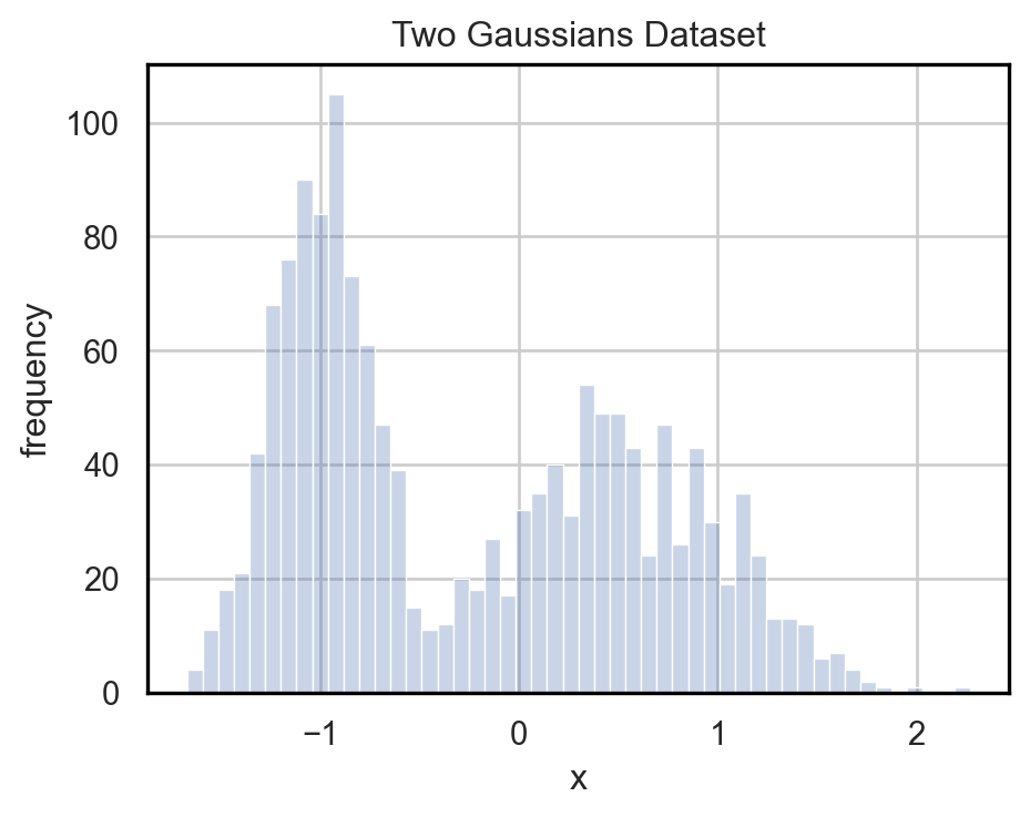
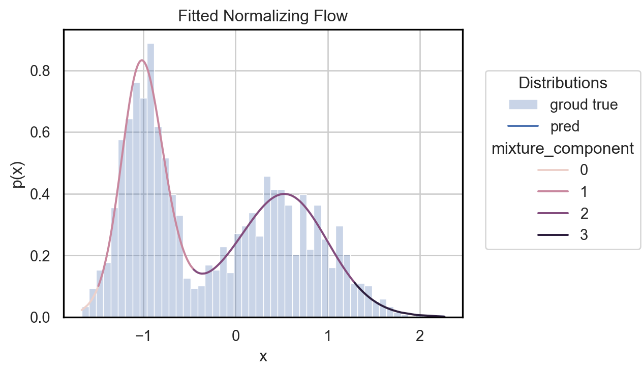
Suppose we are given a 1D dataset, as shown in Fig. [2.a]. We can fit an NF to the underlying probability distribution \(p(x)\) of the dataset. To successfully learn the density of the dataset, we need a base distribution (let’s say a Beta distribution parameterized by \(\alpha = 2\) and \(\beta = 5\)) and a functional definition for our flow. In this case, let’s use the cumulative distribution function of a Gaussian Mixture Model (GMM) with 4 different components:
model = NormalizingFlow(
    prior=Beta(2.0, 5.0),
    flows=nn.ModuleList([
        GMMFlow(n_components=4, dim=1)
    ]),
)
optimizer = optim.AdamW(model.parameters(), lr=5e-3, weight_decay=1e-5)
With these ingredients, we can train the model by minimizing the negative log-likelihood using stochastic gradient descent (SGD):
for epoch in range(epochs):
    model.train()

    for idx, (x, y) in enumerate(dataloader):
        optimizer.zero_grad()
        log_prob, _ = model(x)
        loss = -log_prob.mean()  # nll
        loss.backward()
        nn.utils.clip_grad_norm_(model.parameters(), 1)
        optimizer.step()
Note that no labels are used for training, as the objective is to directly maximize the predicted density of the dataset.
Figure 2 shows the learned density and how the 4 different components are used to correctly model \(p(x)\). While the same results might be achieved by using only 2 components, in the general case, the minimum number of needed components is not known a priori; thus using a larger number of components is a good practice.
Finally, Figure 4 demonstrates how the learned model is able to map a dataset coming from an unknown density to the Beta distributin over-defined.

Full code is contained in the following notebook.
2D Training Example
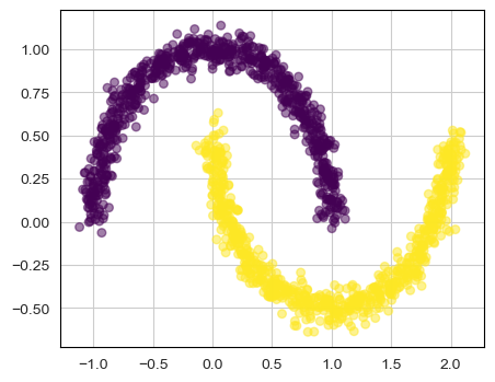
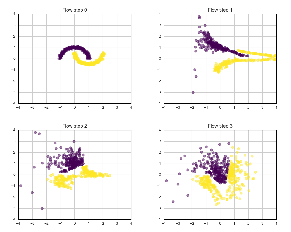
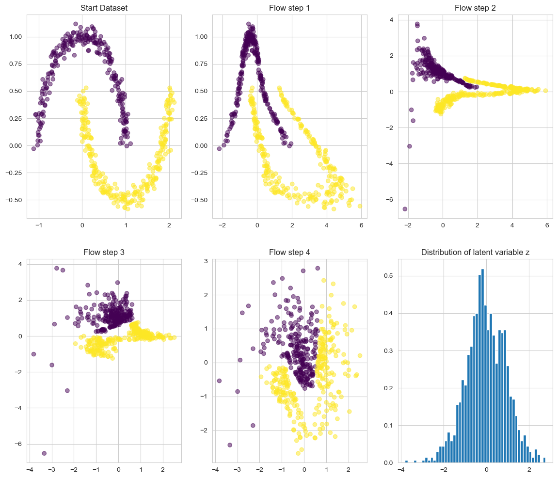
Consider a more intricate dataset, such as the famous 2 Moon dataset depicted in Fig. [3.a]. The objective here is to map samples from this dataset into a latent variable that conforms to a Gaussian distribution.
In this context, relying solely on the cumulative distribution function of a Gaussian Mixture model as NF formulation may not provide the necessary expressiveness. While Neural Networks serve as powerful function approximators, they do not inherently guarantee the conditions required by a normalizing flow. Furthermore, computing the determinant of a linear layer within a neural network is computationally expensive.
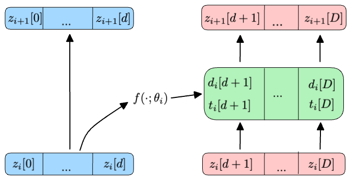
In recent years, Coupling layers [4] have emerged as effective solutions for Normalizing Flows. They prove efficient both during sampling and training, while delivering competitive performances. The fundamental idea involves splitting the input variables of the i-th layer into equally sized groups:
- The first group of input variables (\(z_i[0], ..., z_i[d]\)) is considered constant during the i-th layer1.
- The second group of parameters (\(z_{i}[d+1], ..., z_{i}[D]\)) undergoes transformation by a Neural Network that depends solely on \(z_{i}[\leq d]\).
Mathematically, we can represent the transformation applied to all input variables in the i-th layer as:
\[ \begin{align*} z_{i+1}[0], ..., z_{i+1}[d] & = z_{i}[0], ..., z_{i}[d] \\ d_{i}[d+1], ..., d_{i}[D], t_{i}[d+1], ..., t_{i}[D] & = f(z_{i}[0], ..., z_{i}[d]; \theta_{i}) \\ z_{i+1}[d+1], ..., z_{i+1}[D] & = (z_{i}[d+1] \cdot d_{i}[d+1]) + t_{i}[d+1], ..., (z_{i}[D] \cdot d_{i}[D]) + t_{i}[D] \end{align*} \]
where \(f(\cdot; \theta_i)\) is any neural network. Intuitively, a coupling layer is akin to an autoregressive layer, where the autoregressive mask only permits \(z_{i+1}[>d]\) to depend on \(z_{i}[\leq d]\).
As shown in Figure 7 and Figure 8, the beauty of coupling layers lies in the ease of inverting their transformation. Given the initial conditiokn \(z_{i+1}[\leq d] = z_{i}[\leq d]\), it is possible to derive the affine parameters \(d_{i}[> d]\) and \(t_{i}[> d]\) by directly applying \(f(\cdot; \theta_i)\) to \(z_{i+1}[\leq d]\).

By construction, the Jacobian matrix of any such layer is lower triangular, following the structure:
\[ J_{z_{i+1}}(z_{i}) = \begin{bmatrix} \mathbf{I} & \mathbf{O} \\ \mathbf{A} & \mathbf{D} \\ \end{bmatrix}. \]
Here, \(\mathbf{I}\) is an identity matrix of size \(d \times d\), \(\mathbf{O}\) is a zeros matrix of size \(d \times (D-d)\), \(\mathbf{A}\) is a full matrix of size \((D-d) \times d\) and \(\mathbf{D}\) is a diagonal matrix of shape \((D-d) \times (D-d)\). The determinant of such a matrix is formed by the product of the diagonal elements of \(\mathbf{D}\), making it efficient to compute.
Figure 9 illustrates the dynamics of a NF trained on a 2 Moon dataset. Note how the final latent space (step 4) conforms to a Gaussian distribution.
Finally, a simple implementation of a coupling layer in pytorch is proviceded as follow:
class CouplingFlow(nn.Module):
    def __init__(
        self,
        dim: int,
        hidden_dim: int,
        mask: Tensor,
    ) -> None:
        super().__init__()
        assert dim % 2 == 0, "dim must be even"
        assert dim == mask.size(-1), "mask dimension must equal dim"

        self.dim = dim
        self.hidden_dim = hidden_dim
        self.register_buffer("mask", mask)

        self.net = nn.Sequential(
            nn.Linear(dim, hidden_dim),
            nn.LeakyReLU(),
            nn.Linear(hidden_dim, dim),
        )

    def forward(self, x: Tensor) -> Tensor:
        x_masked = x * self.mask
        output = self.net(x_masked)
        log_d, t = output.chunk(2, dim=-1)
        z = x_masked + ((1 - self.mask) * (x * torch.exp(log_d) + t))
        return z

    def log_abs_det_jacobian(
        self,
        x: Tensor,
        z: Tensor,
    ) -> Tensor:
        x_masked = x * self.mask
        log_d, t = self.net(x_masked).chunk(2, dim=-1)
        return log_d.sum(dim=-1)
Credits
The content of this post is based on the lectures and code of Pieter Abbeel, Justin Solomon and Karpathy’s tutorial. Moreover, I want to credit Lil’Long and Eric Jang for their amazing tutorials. For example, the pioneering work done by Dinh et. al. is the first to leverage transformations with triangular matrix for efficent determinatnt computation.
References
Footnotes
Here we introduce the notation \(z_{i}[d]\) as indicating the \(d\) dimention of the latent variable at the i-th layer of a flow (\(z_{i}\)).↩︎