Gradinet Descent and Backpropagation
Most deep learning algorithm relay on the idea of learning some useful information from the data to solve a specific task. That is, instead of explicitly define every single instruction that a program has to perform, in machine learning, we specify an optimization routine that a program executes over a set of examples to improve its performances. By executing the optimization algorithm, a machine automatically navigates the solution space to find the best “program” that solve the given task starting from a random state: \(\mathbf{\theta}\). It is expectable that the initial program obtained based on the random state would not perform well on the chosen task, however, by iterating over the dataset, we can adjust \(\mathbf{\theta}\) until we obtain an optimal solution.
Gradient Descent
One of the most common learning algorithm is known as Gradient Descent or Stochastic Gradient Descent (SGD) [1]. The core idea of SGD is to iteratively evaluate the difference between the obtained prediction of the model (\(y_{\theta}\)), and, the desired output (\(y\)) utilizing a loss function \(\mathcal{L}(y_{\mathbf{\theta}}, y)\). Once the difference is known, it is possible to adjust \(\theta\) to reduce the difference or prediction error.
Formally, SGD is composed of 3 main steps:
- evaluate the loss function: \(\mathcal{L}(y_{\mathbf{\theta}}, y)\),
- compute the gradient of the loss function w.r.t. the model parameters: \(\nabla \mathcal{L}_{\theta} = \frac{\partial \mathcal{L}(y_{\theta}, y)}{\partial \theta}\),
- update the model parameters (or solution) to decrease the loss function: \(\mathbf{\theta} = \mathbf{\theta} - \eta \nabla \mathcal{L}_{\theta}\).
As it is possible to notice, such a learning algorithm requires a loss function that is continuous and differentiable; otherwise, it is not applicable. However, over the years, many efficient and effective loss functions have been proposed.
Backpropagation
Computing the analytical gradients for a deep learning algorithm might not be easy, and it is definitely an error-prone procedure. Luckily, over the years mathematicians manage to programmatically compute the derivate of most of the functions with a procedure known as algorithmic differentiation. The application of algorithmic differentiation to compute the SGD is known as backpropagation.
Supposing to have the current function \(f(x,y,z) = (x + y) \cdot z\). It is possible to simplify it’s computation defining an intermediate function:
\[ q(x, y) = x + y \Rightarrow f(q, z) = q \cdot z. \]
Knowing that:
- \(\frac{\partial f}{\partial q} = z\)
- \(\frac{\partial f}{\partial z} = q\)
- \(\frac{\partial q}{\partial x} = 1\)
- \(\frac{\partial q}{\partial y} = 1\)
we can compute \(\frac{\partial f}{\partial x}\) by chain rule:
\[ \frac{\partial f}{\partial x} = \frac{\partial f}{\partial q} \cdot \frac{\partial q}{\partial x}. \]
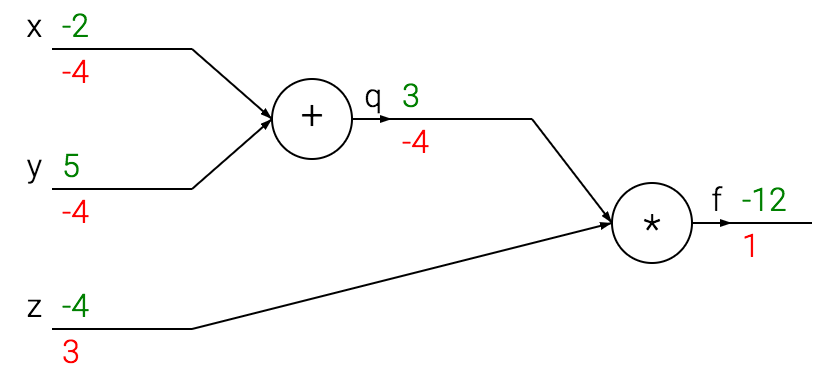
This operation can be seen even as a computational graph, where each node represent an operation ; and using backpropagation it is possible to compute the gradient of function \(f\) w.r.t. its input variable \(x\) and \(y\):

It has to be noted that, backpropagation is a local and global process. It is local since a gate, during the forward pass, can compute:
- its output value: \(q = x + y = 3\),
- as well as its local gradient (the gradient of its input w.r.t. its output): \(\frac{\partial q}{\partial x} = 1\) and \(\frac{\partial q}{\partial y} = 1\).
It is global since, a gate need to know the gradient of its output node in order to evaluate the chain rules: \(\frac{\partial f}{\partial q}\). The gradient of its ouput is known only during the backward pass, thus all the local computations need to be stored in memory; thus require a lot of memory.
The backward pass start by computing: \(\frac{f}{\partial f} = 1\). Then, knowing that \(\frac{\partial f}{\partial q} = z\) and \(\frac{\partial f}{\partial q} = \frac{f}{\partial f} \frac{\partial f}{\partial q} = 1 \cdot -4 = -4\). Similarly, \(\frac{\partial f}{\partial z} = q\) and \(\frac{\partial f}{\partial z} = \frac{f}{\partial f} \frac{\partial f}{\partial z} = 3\). Finally, our goal is to goal is to compute: \[ \frac{\partial f}{\partial x} = \frac{\partial f}{\partial q} \frac{\partial q}{\partial x} = -4 \cdot 1 = -4 \] and, \[ \frac{\partial f}{\partial y} = \frac{\partial f}{\partial q} \frac{\partial q}{\partial y} = -4 \cdot 1 = -4 \].
Weight Decay
To achieve better generaliation performance it is well known that graient updates needs to be regularized so to have sparse or force small weights magnitude. The two most common regularizations for gradiens are L1-regularization or weight decay [2] (equivalent to the L2-regularization):
\[ \theta_{t+1} = \theta_t - \alpha \frac{\partial f(x; \theta_t)}{\partial \theta_t} - \lambda \theta_t \]
where \(\lambda \theta_t\) stand for weight decay or L2-regularization. However, weight dacay and L2-regularization are equivalent only for SDG, but not for Adam or other adaptive optimizers. Instead of applying the same learning rate to all parameters, Adam apply a different learning rate to each parameters proportional to the update signals they recently recevied (a.k.a proportional to the recent gradients). As Adam uses a different learning rate per each parameters, it means that L2-regularization is not only affected by \(\lambda\) but also from the learning rate and the momentum. Thus, Adam requires a bigger regularizer coefficent to achieve comparable performance as SGD.